Rereading the Transformer Upgrade Path (1): Tracing Sinusoidal Positional Encoding to Its Source

Sources. This article primarily draws on Jianlin Su’s “Transformer Upgrade Path 1: Tracing Sinusoidal Positional Encoding to Its Source”, together with the Transformer and RoFormer papers.

Thirty-second summary. A sin/cos pair can be viewed as a hand rotating around the unit circle. Every step forward by one token rotates the hand by a fixed angle, so the distance between two positions becomes a phase difference between two hands. One hand repeats periodically, so the full encoding places many hands with different speeds side by side. The most elegant feature of sinusoidal positional encoding is not that it “assigns different numbers to positions,” but that it turns translation along a sequence into rotation in a representation space.

We will repeatedly use the following notation:

Symbol	Meaning
$m,n$	Absolute position indices of two tokens
$\Delta=m-n$	Relative displacement between the two positions
$d$	Total dimensionality of the position vector, usually even
$i$	Index of the $i$-th sin/cos dimension pair
$\theta_i$	Radians rotated by the $i$-th hand for each token step
$\lambda_i=2\pi/\theta_i$	Number of token steps required for the $i$-th hand to complete one revolution
$b$	Base of the geometric frequency schedule; the classic Transformer uses $b=10000$
$p_m$	Full position vector at position $m$

1. What Does Self-Attention Lack Without Positional Encoding?

Consider a minimal example: “cat chases dog” and “dog chases cat” contain the same three tokens, but changing their order changes the meaning completely. If a model knows only token content and receives no position-dependent signal, it lacks a coordinate system for distinguishing these two sequences.

More precisely, remove the attention mask, position bias, and positional encoding. Let

$$X=[x_1,x_2,\ldots,x_N]^\top$$

denote a sequence of token representations, and let $P$ be any permutation matrix. Pure self-attention satisfies

$$\operatorname{Attn}(PX)=P\operatorname{Attn}(X).$$

This property is called permutation equivariance, not permutation invariance: if the inputs are permuted, the outputs are permuted in the same way. The model can compare token content, but it has no independent signal for “which position,” “before which token,” or “how many steps apart.”

A decoder’s causal mask already supplies the directional constraint that a token cannot attend to the future, but that constraint is not the coordinate encoding discussed here. Our question is: how can we assign a vector to every position so that the model can distinguish absolute positions and conveniently use relative distances?

The classic Transformer takes the most direct approach and adds a position vector to the token at position $m$:

$$\tilde{x}_m=x_m+p_m.$$

Using different $p_m$ values at different positions breaks the original permutation symmetry. But making every position different is only the minimum requirement.

2. Why Is Making Every Position “Different” Not Enough?

Compare the two position pairs

$$(10,12) \qquad\text{and}\qquad (100,102).$$

Their absolute coordinates are completely different, but both relative displacements equal $-2$. If distinctness were the only goal, random vectors, one-hot encodings, or a learned embedding table would all suffice. A more structured objective is to make it easy for the model to discover that these two pairs share the same relative relationship.

To isolate the geometry supplied by the position vectors, define a simplified positional interaction kernel:

$$K_{\text{pos}}(m,n)=p_m^\top p_n.$$

We would like this kernel to depend only on relative displacement:

$$\boxed{p_m^\top p_n=g(m-n)}.$$

Then, for any global shift $c$,

$$p_{m+c}^{\top}\,p_{n+c} =g((m+c)-(n+c)) =g(m-n).$$

In other words, two position pairs separated by the same distance have the same pure positional similarity.

The boundary of this argument should be explicit: $p_m^\top p_n$ is a simplified object used to isolate positional structure. It is not the complete attention score produced by additive positional encoding. The real score also mixes token content and projection matrices; Section 7 expands it in full.

Moreover, $p_m^\top p_n=g(m-n)$ is a clear and tractable sufficient condition, not a definition that every positional encoding must obey. Our next task is to construct a simple family of vectors that satisfies it.

3. One Clock: How Do Sin/Cos Encode Relative Position?

Start with only two dimensions and place position $m$ on the unit circle:

$$p_m= \begin{bmatrix} \cos(m\theta)\\ \sin(m\theta) \end{bmatrix}.$$

The parameter $\theta$ means “how many radians the clock hand rotates for each token step.” Therefore:

• Position $0$ has angle $0$.
• Position $1$ has angle $\theta$.
• Position $m$ has angle $m\theta$.
• When the position index advances from $m$ to $m+T$, the hand rotates by an additional $T\theta$. If $T\theta=2\pi$, it completes exactly one revolution, so the one-revolution period is $T=2\pi/\theta$.

The quantity that changes is the position index $m$; $\theta$ is the fixed “rotation per step” of this hand. Thus $m\theta$ is the total angle accumulated by the time the hand reaches position $m$. “Completing one revolution” means that the accumulated angle increases by $2\pi$ and the hand returns to the same point on the unit circle. If $2\pi/\theta$ is not an integer, exactly one revolution does not correspond to an integer number of token steps.

For example, let $\theta=\pi/4$:

Position index $m$	Total angle $m\theta$	Corresponding 2D vector $p_m=[\cos(m\theta),\sin(m\theta)]^\top$
0	$0$	$[1,0]^\top$
1	$\pi/4$	$[\sqrt{2}/2,\sqrt{2}/2]^\top$
2	$\pi/2$	$[0,1]^\top$
3	$3\pi/4$	$[-\sqrt{2}/2,\sqrt{2}/2]^\top$

The pairs $(0,2)$ and $(1,3)$ are both separated by two tokens. The angle between each pair of hands is also $2\theta=\pi/2$, so both inner products equal $0$.

In general, the inner product between two position vectors is

$$\begin{aligned} p_m^\top p_n &=\cos(m\theta)\cos(n\theta) +\sin(m\theta)\sin(n\theta)\\ &=\cos((m-n)\theta). \end{aligned}$$

The second step is simply the cosine subtraction identity. Therefore,

$$\boxed{p_m^\top p_n=\cos((m-n)\theta)}.$$

The right-hand side no longer depends on $m$ and $n$ separately; it depends only on the relative displacement $m-n$. The unit circle establishes the correspondence

$$\boxed{\text{position difference}\ \longleftrightarrow\ \text{phase difference}}.$$

The canonical formula orders each coordinate pair as $[\sin,\cos]$, whereas the derivation above uses $[\cos,\sin]$. Swapping the two coordinates changes neither the inner product nor the rotation structure.

This derivation does not imply that sin/cos is the unique solution. It shows that if we seek a two-dimensional representation with fixed length that rotates uniformly with position, sin/cos provides the most natural and simplest family of coordinates.

4. Why Is One Clock Not Enough?

A clock repeats periodically. If $\theta=2\pi/10$, then

$$\begin{aligned} \cos((m+10)\theta) &=\cos(m\theta+2\pi)=\cos(m\theta),\\ \sin((m+10)\theta) &=\sin(m\theta+2\pi)=\sin(m\theta). \end{aligned}$$

Hence,

$$p_{m+10}=p_m.$$

Positions $m$ and $m+10$ land on the same point of the unit circle. At integer positions, this two-dimensional hand has only $10$ distinct phases. Once a sequence contains more than $10$ positions, the phases repeat, so this hand alone cannot distinguish positions separated by $10,20,30,\ldots$ tokens. This does not mean that the entire Transformer can hold only $10$ tokens: the limitation belongs to this deliberately chosen single frequency, while the full encoding combines many hands with different periods.

A $d$-dimensional sinusoidal positional encoding places $d/2$ clocks with different speeds side by side:

$$p_m= \begin{bmatrix} \sin(m\theta_0)\\ \cos(m\theta_0)\\ \sin(m\theta_1)\\ \cos(m\theta_1)\\ \vdots\\ \sin(m\theta_{d/2-1})\\ \cos(m\theta_{d/2-1}) \end{bmatrix}.$$

When one clock returns to its initial phase, the others will usually not reset at the same time. Multiple frequencies therefore provide two benefits:

1. They reduce positional ambiguity caused by a single period.
2. They resolve displacement at several distance scales.

Larger $\theta_i$ values rotate quickly, so adjacent tokens create noticeable phase changes and local displacement is easier to resolve. Smaller $\theta_i$ values rotate slowly and retain gradually changing structure over a longer interval.

Multiple frequencies are not an unconditional guarantee against collisions at arbitrary lengths or under finite numerical precision. Distance information is carried by the joint phase pattern across all dimensions, and the model must still learn how to use that pattern during training.

5. Why Space the Frequencies Geometrically?

The general form of a geometric frequency schedule is

$$\theta_i=b^{-2i/d}.$$

Here $b>1$ is the base that controls the span of the full frequency set. The classic Transformer chooses $b=10000$, giving

$$\theta_i=10000^{-2i/d}, \qquad i=0,1,\ldots,\frac d2-1.$$

The corresponding periods are

$$\lambda_i=\frac{2\pi}{\theta_i} =2\pi\,10000^{2i/d}.$$

For $d=8$, we can see directly how the clocks become progressively slower:

Frequency pair $i$	$\theta_i$	Period $\lambda_i$ (approx.)	Intuition
0	$1$	$6.28$	Rapid change, local emphasis
1	$0.1$	$62.8$	Shorter scale
2	$0.01$	$628$	Longer scale
3	$0.001$	$6283$	Slow change, global emphasis

This is the main value of geometric spacing: a finite number of dimensions can cover logarithmic scales relatively evenly. With an arithmetic frequency schedule, many dimensions may cluster in a narrow absolute range. Geometric spacing instead acts like a multiscale ruler that moves from local detail toward global structure.

Two questions should remain separate:

1. Why sin/cos? Rotations and the angle-subtraction identity make relative displacement appear naturally in positional interactions.
2. Why the base 10000? It is an engineering choice governing frequency range and resolution, not a constant uniquely forced by the preceding identity.

The Transformer paper also gives a direct motivation: for any fixed offset $k$, $\operatorname{PE}_{m+k}$ can be represented as a linear function of $\operatorname{PE}_m$. A fixed function can also generate encodings at positions longer than those seen during training. The latter means only that “the formula can be evaluated”; it does not automatically imply reliable length extrapolation by the model.

6. Distance Behavior of the Multi-Frequency Position Kernel: Oscillatory Decorrelation

First, write the two complete position vectors side by side:

$$p_m= \begin{bmatrix} \sin(m\theta_0)\\ \cos(m\theta_0)\\ \vdots\\ \sin(m\theta_{d/2-1})\\ \cos(m\theta_{d/2-1}) \end{bmatrix}, \qquad p_n= \begin{bmatrix} \sin(n\theta_0)\\ \cos(n\theta_0)\\ \vdots\\ \sin(n\theta_{d/2-1})\\ \cos(n\theta_{d/2-1}) \end{bmatrix}.$$

Their inner product multiplies sin by sin and cos by cos within each frequency pair, then sums over all pairs:

$$\begin{aligned} p_m^\top p_n &=\sum_{i=0}^{d/2-1} \left[ \sin(m\theta_i)\sin(n\theta_i) +\cos(m\theta_i)\cos(n\theta_i) \right]\\ &=\sum_{i=0}^{d/2-1}\cos((m-n)\theta_i). \end{aligned}$$

The last step applies the cosine subtraction identity to every dimension pair. The result says that the full-vector inner product is the sum of all clocks’ “votes” on their phase differences.

Let $\Delta=m-n$ and divide by the number of clocks, $d/2$, to obtain the normalized position kernel

$$\kappa_d(\Delta) =\frac{2}{d}\sum_{i=0}^{d/2-1}\cos(\Delta\theta_i).$$

The normalization gives

$$\kappa_d(0)=1,$$

because when $\Delta=0$, every clock is perfectly aligned and every cosine term equals $1$.

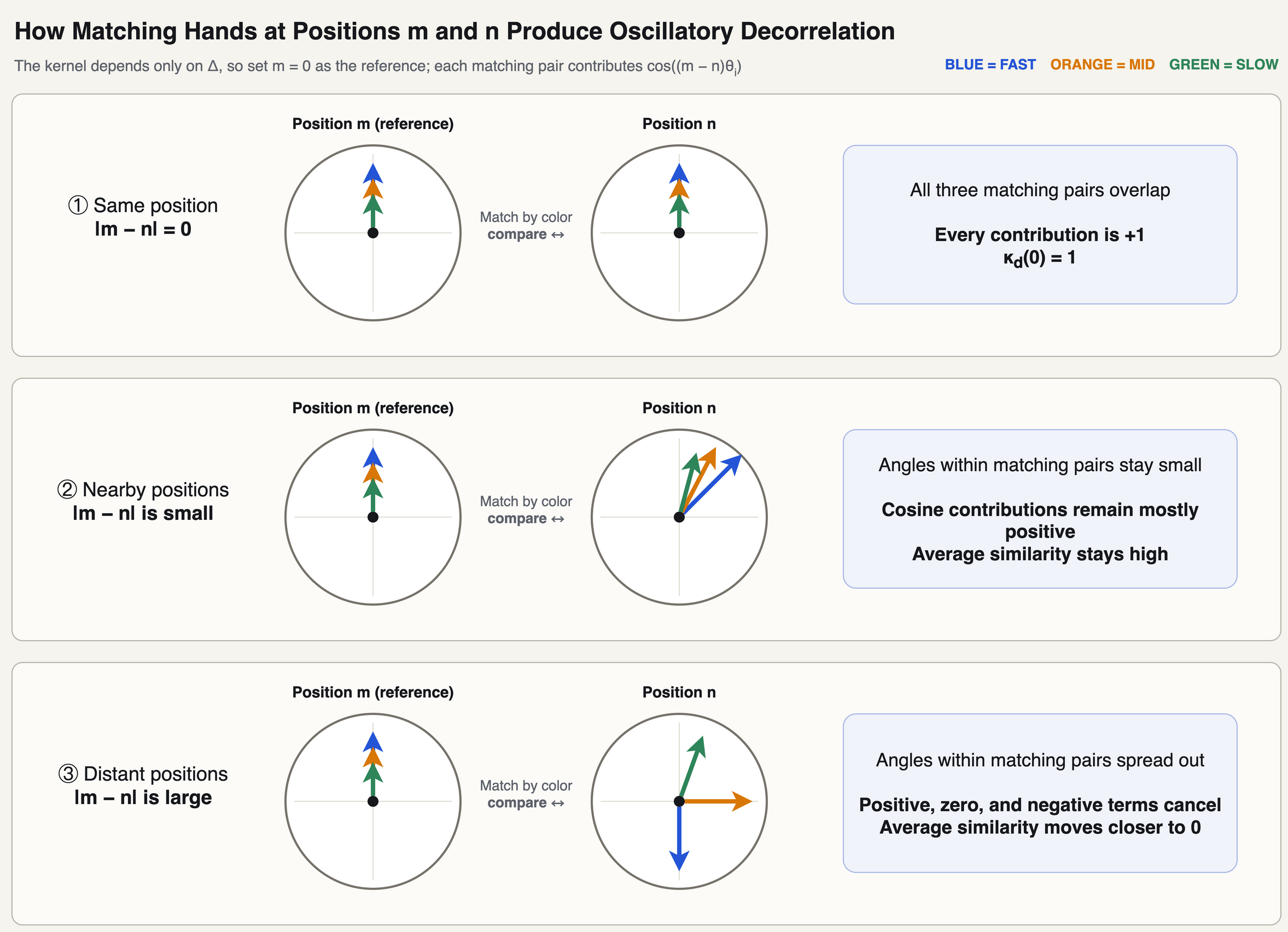
When $|\Delta|$ is small, the phases at different frequencies remain relatively synchronized, so many cosine terms reinforce one another. As distance grows, the phases spread apart and positive and negative terms begin to cancel. Over commonly used distance ranges, this often produces oscillatory decorrelation: distant positions tend to have lower average similarity, but the curve repeatedly rises and falls along the way.

Figure 1 makes this process explicit by drawing the three hands at position $m$ and position $n$ in every row. Because the position kernel depends only on $\Delta=m-n$, we can set $m=0$ as the reference without loss of generality; all three hands on the left then point to 12 o’clock. On the right, the angle between each matching color and the reference direction is determined by $|\Delta|\theta_i$. The cosine of that angle is the inner-product contribution of the corresponding frequency pair.

An important point is that every two-dimensional block remains on the unit circle, so the length of the full position vector is constant:

$$\lVert p_m\rVert=\sqrt{d/2}.$$

As distance grows, the positional encoding itself does not “shrink to zero.” What may become smaller is the normalized inner product $\kappa_d(\Delta)$ between two position vectors. In other words, the average alignment between their directions changes, not their vector lengths.

This trend should not be mistaken for a strict theorem:

With finitely many frequencies, $\kappa_d(\Delta)$ is a finite cosine sum. It is not guaranteed to decrease monotonically with distance, nor can we generally claim that it converges strictly to zero as $|\Delta|\to\infty$.

To study the overall trend of many discrete frequencies, treat the frequency index $t=2i/d$ as a continuous variable on $[0,1]$. From $\theta_i=b^{-2i/d}$, we obtain $\theta(t)=b^{-t}$, and the discrete average can be approximated by

$$\kappa_d(\Delta) \approx\int_0^1\cos(\Delta b^{-t})\,\mathrm{d}t.$$

Here $b$ is the frequency-schedule base defined in Section 5, with the classic value $10000$. The integral can be read as an average over a continuous distribution of clocks with different speeds. As $|\Delta|$ grows, the integrand oscillates between positive and negative values more rapidly as a function of $t$, so its average is more easily cancelled.

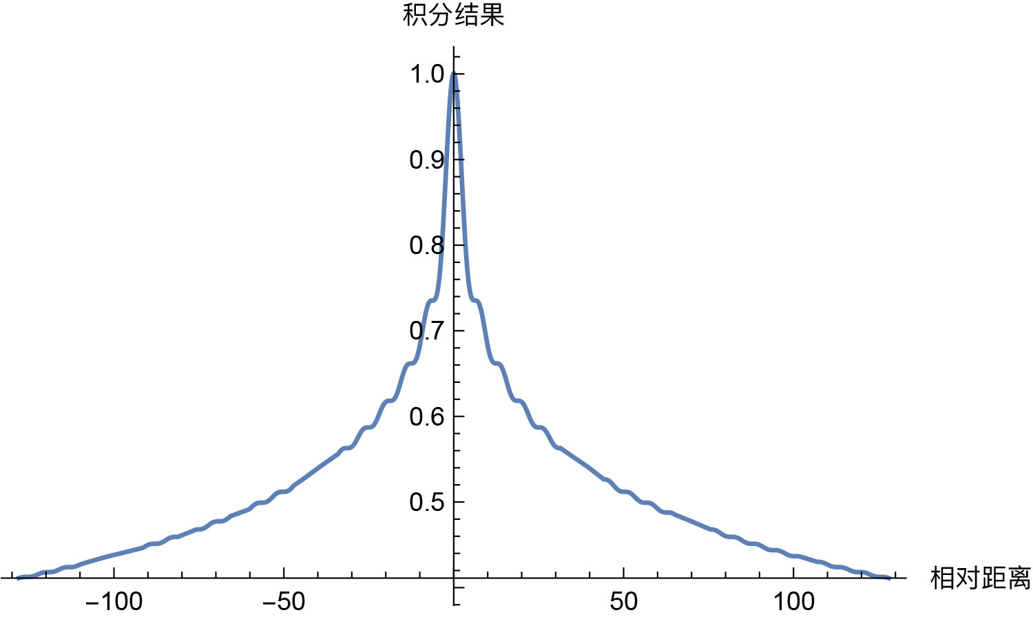
The purpose of this figure is to turn “positive and negative contributions from many frequencies gradually cancel” into a visible continuous curve. It is not evidence that a particular finite-dimensional positional encoding must eventually converge to zero. The schedule $10000^{-t}$ is not the only possible choice either; it is an engineering compromise among local resolution, long-distance variation, and frequency coverage.

Section takeaway: what is often called “long-range decay” is more precisely oscillatory decorrelation. As $|\Delta|$ grows, phases at different frequencies are more likely to spread out, and the normalized inner product tends to be smaller over commonly used distance ranges. A finite cosine sum, however, is neither guaranteed to decrease monotonically nor guaranteed to converge to zero. What changes is the average similarity between two positions, not the length of either position vector.

7. How Does Real Attention Differ from This Simplified Model?

So far, we have studied $p_m^\top p_n$. Now place it back inside real attention.

Ignoring the scaling constant and bias, suppose the Query and Key are computed from tokens after their position vectors have been added:

$$q_m=W_Q(x_m+p_m), \qquad k_n=W_K(x_n+p_n).$$

Let

$$A=W_Q^\top W_K.$$

The attention score then expands exactly as

$$\begin{aligned} q_m^\top k_n &=(x_m+p_m)^\top A(x_n+p_n)\\ &=\underbrace{x_m^\top Ax_n}_{\text{content--content}} +\underbrace{x_m^\top Ap_n}_{\text{content--position}} +\underbrace{p_m^\top Ax_n}_{\text{position--content}} +\underbrace{p_m^\top Ap_n}_{\text{position--position}}. \end{aligned}$$

Therefore, using sinusoidal positional encoding does not automatically make the real score a function of $m-n$ alone. The earlier identity

$$p_m^\top p_n=g(m-n)$$

first isolates the pure positional interaction, then examines the simplest case $A=I$ to reveal the structure supplied by the encoding itself.

Directly expanding the attention score also exposes the boundary clearly. When $A$ is a general matrix, the pure positional term $p_m^\top A p_n$ need not depend only on $m-n$; the other three terms additionally mix content and position. The kernel in Section 6 is therefore a simplified tool for analyzing encoding geometry, not an equivalent description of complete attention behavior.

A more accurate conclusion is:

Sinusoidal positional encoding gives the model a relative phase structure that it can exploit, but it does not dictate how a trained model must use that structure.

8. What Does This Explanation Establish—and What Does It Not?

It establishes or directly demonstrates that:

1. A sin/cos pair forms two-dimensional rotation coordinates.
2. The inner product within one frequency pair is exactly $\cos((m-n)\theta)$.
3. A fixed positional offset corresponds to a rotation independent of the absolute position.
4. Multiple frequencies extend this structure across several distance scales.
5. Geometric frequencies produce an oscillatory decorrelation trend under the continuous approximation.

It does not establish that:

1. Sinusoidal PE is the only positional encoding.
2. Sinusoidal PE is the optimal positional encoding.
3. The base $10000$ is theoretically mandatory or optimal.
4. A finite-dimensional inner product decreases strictly monotonically with distance.
5. The real attention score of additive sinusoidal PE depends only on relative position.
6. Being able to evaluate encodings at longer positions guarantees reliable length extrapolation.

The real value of this analysis is not to prove that “Google’s formula is irreplaceable.” It demonstrates a reusable way of thinking: first specify the structure we want a positional representation to have, then find a simple explicit construction, and finally inspect the additional properties and assumptions that come with it.

9. Extension: Why Does This Idea Lead Naturally to RoPE?

The principle that “relative displacement becomes phase difference” can enter attention through a different mechanism. This is the natural starting point for understanding RoPE.

Traditional sinusoidal PE adds a position vector to a token representation:

$$x_m\longmapsto x_m+p_m.$$

RoPE instead applies the position-dependent rotation directly to content-derived Queries and Keys. For one two-dimensional frequency block, let $R_m$ denote the rotation at position $m$:

$$\tilde q_m=R_mq_m, \qquad \tilde k_n=R_nk_n.$$

Their inner product is

$$\begin{aligned} \tilde q_m^\top\tilde k_n &=q_m^\top R_m^\top R_nk_n\\ &=q_m^\top R_{n-m}k_n. \end{aligned}$$

Full RoPE uses two-dimensional rotation blocks with different frequencies across dimension pairs. Position enters the Q/K inner product explicitly through $R_{n-m}$, while the complete score still depends on the content vectors $q_m$ and $k_n$.

The two methods therefore share the mathematical core that relative displacement corresponds to phase difference, but their mechanisms differ:

• Sinusoidal PE adds an absolute position vector at the input, after which position and content pass through the projections together.
• RoPE rotates content directly in Q/K space, making relative rotation explicit in the score.

10. Quick Reference

Question	Shortest answer
Why do we need positional encoding?	Position-free self-attention is permutation equivariant and lacks an independent coordinate for sequence order.
Why is making every position different not enough?	We also want the model to recognize easily that $(10,12)$ and $(100,102)$ share the same relative relationship.
Why use sin/cos?	Unit-circle rotations make the inner product depend only on position difference through the angle-subtraction identity.
Why pair every two dimensions?	Two dimensions are exactly enough to represent the two coordinates of one rotating hand.
Why use many frequencies?	A single frequency repeats periodically; multiple frequencies reduce ambiguity and provide several scales.
Why use geometric frequencies?	They cover logarithmic scales relatively evenly with a finite number of dimensions.
Is oscillatory decorrelation strictly monotonic?	No. A finite-dimensional inner product is an oscillatory cosine sum and only shows a decorrelation trend over commonly used ranges.
Is $10000$ theoretically mandatory?	No. It is an engineering choice governing frequency range and resolution.
Does real attention depend only on relative distance?	No. With additive PE, the score contains four kinds of content-position interaction.
How is this related to RoPE?	Both use phase differences; RoPE places the rotation directly inside the Q/K inner product.

The single most important sentence to remember is:

Sinusoidal positional encoding does not use trigonometric functions merely to “number positions.” It uses many clocks with different speeds to represent relative displacement as a multiscale phase difference.

References and Image Sources

1. Vaswani, A. et al. (2017). Attention Is All You Need, §3.5.
2. Jianlin Su (2021). “Transformer Upgrade Path 1: Tracing Sinusoidal Positional Encoding to Its Source”. The motivating questions, relative-position inner product, and continuous-frequency approximation in this article begin from that post. The pedagogical sequence has been reorganized, and a direct attention-score decomposition replaces the Taylor expansion.
3. Su, J. et al. (2021). RoFormer: Enhanced Transformer with Rotary Position Embedding.
4. Figure 1 is an author-created mechanism diagram. Figure 2 is taken from Jianlin Su’s post above and reproduced unaltered under the site’s CC BY-NC-ND 2.5 CN notice; open the image to view the source file.