Rereading the Transformer Upgrade Path (2): How RoPE Writes Relative Position into Attention

Sources. This article primarily draws on Jianlin Su’s “Transformer Upgrade Path 2: Rotary Position Embedding That Combines the Best of Both Worlds”, together with the RoFormer, Linear Transformer, and Performer papers.

Thirty-second summary. In the previous article, “Rereading the Transformer Upgrade Path (1): Tracing Sinusoidal Positional Encoding to Its Source”, every sin/cos pair acts like a “position clock” that generates a hand for each position. RoPE goes one step further: instead of adding a position vector to a token, it uses the angle associated with that position to rotate the content-derived Query and Key directly. Position $m$ rotates by $m\theta$, and position $n$ by $n\theta$; when their inner product is taken, the shared absolute rotation cancels, leaving only $n-m$. In standard attention, this relative rotation enters the score before softmax. In linear attention, the computational reordering that aggregates Keys and Values first can be preserved as long as the rotations still act separately on the Query and Key. However, “the computation remains linear” does not mean “the weights remain nonnegative and sum to one.” These are two separate questions.

We will repeatedly use the following notation:

Symbol	Meaning
$m,n$	Absolute positions of the Query and Key
$\Delta=m-n$	Displacement of the Query relative to the Key
$x_m$	Token representation at position $m$
$q_m,k_n,v_n$	Query, Key, and Value before positional information is introduced
$d_h$	Query/Key dimensionality of one attention head, assumed even in this article
$R(\alpha)$	Matrix that rotates a vector counterclockwise by $\alpha$ in the two-dimensional plane
$R_m$	Block matrix that rotates every dimension pair in a complete attention head by $m\theta_i$
$\theta_i$	Radians rotated by the $i$-th dimension pair for each token step
$\phi,\varphi$	Feature maps applied to Queries and Keys in linear attention

1. What Gap in Sinusoidal PE Is RoPE Trying to Fill?

First, put positional encoding aside. Standard self-attention produces three groups of vectors from token representations:

$$q_m=W_Qx_m, \qquad k_n=W_Kx_n, \qquad v_n=W_Vx_n.$$

A Query can be understood as “what position $m$ is looking for,” a Key as “which features position $n$ can be found by,” and a Value as the information actually retrieved after that position has been selected. Their inner product

$$s_{m,n}=q_m^\top k_n$$

determines how well the Query and Key match.

The problem is that if neither $q_m$ nor $k_n$ carries position, then this match compares only content and does not know how many steps separate the two tokens.

The previous article introduced Sinusoidal positional encoding, which first constructs a position vector $p_m$ and then adds it to the token representation. To describe additive PE and RoPE in the same language, write “adding a position vector” as a position-dependent transformation:

$$F_{\mathrm{add}}(x_m,m)=x_m+p_m.$$

The second argument $m$ tells the function which $p_m$ to use. Projecting the transformed tokens into Queries and Keys gives

$$\begin{aligned} \hat q_m &=W_QF_{\mathrm{add}}(x_m,m) =q_m+W_Qp_m,\\ \hat k_n &=W_KF_{\mathrm{add}}(x_n,n) =k_n+W_Kp_n. \end{aligned}$$

Now expand their inner product without skipping any terms:

$$\begin{aligned} \hat q_m^\top\hat k_n ={}&q_m^\top k_n +q_m^\top W_Kp_n\\ &+(W_Qp_m)^\top k_n +(W_Qp_m)^\top(W_Kp_n). \end{aligned}$$

The four terms are content—content, content—position, position—content, and position—position. The previous article showed that the Sinusoidal vectors themselves have a clean relative-phase structure—for example, $p_m^\top p_n$ depends only on $m-n$. But the complete score above also passes through $W_Q,W_K$ and mixes in the other three terms, so it is not forced into a form in which position appears only through $m-n$.

This naturally suggests the next step. If position ultimately exists to affect the Query—Key comparison, can we define a more suitable position transformation directly on the Query and Key? Denote these two transformations by

$$q_m^{\mathrm{pos}}=F_Q(q_m,m), \qquad k_n^{\mathrm{pos}}=F_K(k_n,n).$$

We want them to satisfy

$$\boxed{ F_Q(q_m,m)^\top F_K(k_n,n) =g(q_m,k_n,m-n) }.$$

The right-hand side still depends on the content of the Query and Key. The only restriction is on the position variables: they may appear only through $m-n$. RoPE’s concrete choice is to let both $F_Q$ and $F_K$ use rotations determined by position.

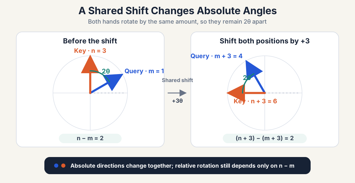
This objective has an intuitive test. If both tokens are shifted backward by $c$ positions, their relative distance does not change:

$$(m+c)-(n+c)=m-n.$$

We therefore also want the content match to remain unchanged after this shared shift. All that remains is to construct a simple transformation with this property.

2. First, Understand Two-Dimensional Rotation Step by Step

2.1 What Exactly Does a Rotation Matrix Do?

In the two-dimensional plane, a vector

$$u= \begin{bmatrix} u_1\\ u_2 \end{bmatrix}$$

becomes

$$R(\alpha)u = \begin{bmatrix} \cos\alpha&-\sin\alpha\\ \sin\alpha&\cos\alpha \end{bmatrix} \begin{bmatrix} u_1\\ u_2 \end{bmatrix} = \begin{bmatrix} u_1\cos\alpha-u_2\sin\alpha\\ u_1\sin\alpha+u_2\cos\alpha \end{bmatrix}$$

after a counterclockwise rotation by $\alpha$.

For example, take $u=[1,0]^\top$, which initially points along the positive horizontal axis. After a rotation by $\pi/2$,

$$R(\pi/2) \begin{bmatrix} 1\\0 \end{bmatrix} = \begin{bmatrix} 0&-1\\1&0 \end{bmatrix} \begin{bmatrix} 1\\0 \end{bmatrix} = \begin{bmatrix} 0\\1 \end{bmatrix},$$

so it now points along the positive vertical axis. Rotation changes the direction of a vector, not its length.

2.2 Why Does the Transpose Equal the Reverse Rotation?

Transposing the rotation matrix swaps its rows and columns:

$$R(\alpha)^\top = \begin{bmatrix} \cos\alpha&\sin\alpha\\ -\sin\alpha&\cos\alpha \end{bmatrix}.$$

On the other hand,

$$\cos(-\alpha)=\cos\alpha, \qquad \sin(-\alpha)=-\sin\alpha,$$

so

$$R(-\alpha) = \begin{bmatrix} \cos\alpha&\sin\alpha\\ -\sin\alpha&\cos\alpha \end{bmatrix}.$$

The two matrices are identical entry by entry. Therefore,

$$\boxed{R(\alpha)^\top=R(-\alpha)}.$$

The geometry is just as simple: after rotating a hand by $\alpha$, restoring it to its original direction requires a rotation by $-\alpha$.

2.3 Why Can Two Consecutive Rotations Add Their Angles?

First rotating by $\beta$ and then by $\alpha$ corresponds to the matrix product

$$R(\alpha)R(\beta).$$

To expose every term, temporarily abbreviate $\cos\alpha,\sin\alpha$ as $c_\alpha,s_\alpha$, and $\cos\beta,\sin\beta$ as $c_\beta,s_\beta$:

$$\begin{aligned} R(\alpha)R(\beta) &= \begin{bmatrix} c_\alpha&-s_\alpha\\ s_\alpha&c_\alpha \end{bmatrix} \begin{bmatrix} c_\beta&-s_\beta\\ s_\beta&c_\beta \end{bmatrix}\\ &= \begin{bmatrix} c_\alpha c_\beta-s_\alpha s_\beta &-(c_\alpha s_\beta+s_\alpha c_\beta)\\ s_\alpha c_\beta+c_\alpha s_\beta &c_\alpha c_\beta-s_\alpha s_\beta \end{bmatrix}. \end{aligned}$$

Now apply the angle-sum identities for sine and cosine:

$$\begin{aligned} \cos(\alpha+\beta) &=c_\alpha c_\beta-s_\alpha s_\beta,\\ \sin(\alpha+\beta) &=s_\alpha c_\beta+c_\alpha s_\beta. \end{aligned}$$

The product above becomes

$$R(\alpha)R(\beta) = \begin{bmatrix} \cos(\alpha+\beta)&-\sin(\alpha+\beta)\\ \sin(\alpha+\beta)&\cos(\alpha+\beta) \end{bmatrix} =R(\alpha+\beta).$$

Hence,

$$\boxed{R(\alpha)R(\beta)=R(\alpha+\beta)}.$$

If there is only one sentence to remember, it is this: rotations multiply; their angles add.

3. Why Does the Core of RoPE Fit in One Line?

Now take one two-dimensional Query and Key:

$$q_m= \begin{bmatrix} q_1\\q_2 \end{bmatrix}, \qquad k_n= \begin{bmatrix} k_1\\k_2 \end{bmatrix}.$$

Choose a fixed per-step rotation angle $\theta$. At position $m$, RoPE rotates the Query by $m\theta$; at position $n$, it rotates the Key by $n\theta$:

$$\tilde q_m=R(m\theta)q_m, \qquad \tilde k_n=R(n\theta)k_n.$$

Take the inner product of the rotated vectors:

$$\begin{aligned} \tilde q_m^\top\tilde k_n &=(R(m\theta)q_m)^\top(R(n\theta)k_n)\\ &=q_m^\top R(m\theta)^\top R(n\theta)k_n\\ &=q_m^\top R(-m\theta)R(n\theta)k_n\\ &=q_m^\top R((n-m)\theta)k_n. \end{aligned}$$

The three steps use, respectively:

1. $(AB)^\top=B^\top A^\top$;
2. $R(\alpha)^\top=R(-\alpha)$;
3. $R(\alpha)R(\beta)=R(\alpha+\beta)$.

Only $n-m$ remains as a position variable in the final expression:

$$\boxed{ \tilde q_m^\top\tilde k_n =q_m^\top R((n-m)\theta)k_n }.$$

Although the Query and Key are each rotated according to their absolute positions $m,n$, when they meet in the inner product they see only their relative position.

If both positions are shifted by $c$, then similarly

$$\begin{aligned} R((m+c)\theta)^\top R((n+c)\theta) &=R(-(m+c)\theta)R((n+c)\theta)\\ &=R((n-m)\theta). \end{aligned}$$

The shared $c$ disappears. This is the matrix form of “a global shift does not change a relative relationship.”

4. What Does “Rotating Content” Actually Change?

The previous section proved that position appears only through $m-n$, but it has not yet answered a more intuitive question: for the same Query and Key, why does changing the relative position change their matching score?

Let

$$\Delta=m-n.$$

Because $n-m=-\Delta$, the two-dimensional RoPE score can be written as

$$q_m^\top R(-\Delta\theta)k_n.$$

To keep every step visible, first write out the two factors on the right:

$$k_n= \begin{bmatrix} k_1\\k_2 \end{bmatrix},$$

and

$$\begin{aligned} R(-\Delta\theta) &= \begin{bmatrix} \cos(-\Delta\theta)&-\sin(-\Delta\theta)\\ \sin(-\Delta\theta)&\cos(-\Delta\theta) \end{bmatrix}\\ &= \begin{bmatrix} \cos(\Delta\theta)&\sin(\Delta\theta)\\ -\sin(\Delta\theta)&\cos(\Delta\theta) \end{bmatrix}. \end{aligned}$$

The second equality uses the fact that cosine is even and sine is odd: $\cos(-x)=\cos x$ and $\sin(-x)=-\sin x$.

First multiply the matrix and the vector:

$$\begin{aligned} R(-\Delta\theta)k_n &= \begin{bmatrix} \cos(\Delta\theta)&\sin(\Delta\theta)\\ -\sin(\Delta\theta)&\cos(\Delta\theta) \end{bmatrix} \begin{bmatrix} k_1\\k_2 \end{bmatrix}\\ &= \begin{bmatrix} k_1\cos(\Delta\theta)+k_2\sin(\Delta\theta)\\ -k_1\sin(\Delta\theta)+k_2\cos(\Delta\theta) \end{bmatrix}. \end{aligned}$$

Now write the transposed Query explicitly as a row vector:

$$q_m^\top= \begin{bmatrix} q_1&q_2 \end{bmatrix}.$$

The inner product can then be evaluated one line at a time:

$$\begin{aligned} q_m^\top R(-\Delta\theta)k_n &= \begin{bmatrix} q_1&q_2 \end{bmatrix} \begin{bmatrix} k_1\cos(\Delta\theta)+k_2\sin(\Delta\theta)\\ -k_1\sin(\Delta\theta)+k_2\cos(\Delta\theta) \end{bmatrix}\\ &=q_1[k_1\cos(\Delta\theta)+k_2\sin(\Delta\theta)]\\ &\quad+q_2[-k_1\sin(\Delta\theta)+k_2\cos(\Delta\theta)]\\ &=q_1k_1\cos(\Delta\theta) +q_1k_2\sin(\Delta\theta)\\ &\quad-q_2k_1\sin(\Delta\theta) +q_2k_2\cos(\Delta\theta)\\ &=(q_1k_1+q_2k_2)\cos(\Delta\theta)\\ &\quad+(q_1k_2-q_2k_1)\sin(\Delta\theta). \end{aligned}$$

The RoPE score therefore contains two parts:

$$\boxed{ \underbrace{(q_1k_1+q_2k_2)}_{\text{original same-direction match}} \cos(\Delta\theta) + \underbrace{(q_1k_2-q_2k_1)}_{\text{cross-coordinate match}} \sin(\Delta\theta) }.$$

The easiest misconception here is to imagine RoPE as “multiplying the original dot product by a distance cosine.” Only the first term has that form. The second term also cross-compares the first coordinate of the Query with the second coordinate of the Key, and the second coordinate of the Query with the first coordinate of the Key.

What does this expression actually say? Two controlled experiments make it concrete. To keep the rotations easy to calculate mentally, temporarily take $\theta=\pi/2$, so a one-position difference means a $90^\circ$ rotation. This is a toy setting chosen to magnify the mechanism, not the only frequency used by a real model.

Experiment	Query $q$	Original Key $k$	$\Delta$	Rotated Key $R(-\Delta\theta)k$	RoPE score
A1	$[1,0]$	$[1,0]$	$0$	$[1,0]$	$1$
A2	$[1,0]$	$[1,0]$	$1$	$[0,-1]$	$0$
B1	$[1,0]$	$[0,1]$	$0$	$[0,1]$	$0$
B2	$[1,0]$	$[0,1]$	$1$	$[1,0]$	$1$

Start with experiment A. The content vectors are identical in both rows; only the relative position changes:

$$\begin{aligned} \Delta=0:&\quad [1,0]\,[1,0]^\top=1,\\ \Delta=1:&\quad [1,0]\,[0,-1]^\top=0. \end{aligned}$$

Thus even when the content is unchanged, relative position rotates the Key first and then changes how well it matches the Query.

Now consider experiment B. The Query and Key are initially orthogonal, so their score at the same position is $0$. When $\Delta=1$, $R(-\pi/2)$ turns the Key from $[0,1]$ into $[1,0]$, exactly aligning it with the Query, and the score becomes $1$.

These examples make only one point: RoPE lets relative position determine the coordinate directions in which two pieces of content are compared. It does not add a fixed reward or penalty for distance, nor does it guarantee that the score decreases with distance.

A real attention head uses many different $\theta_i$ values at once, while $q,k$ are content vectors learned by the model. The position difference determines how each coordinate pair rotates; the content determines whether those rotated coordinates match. The results from all dimensions are then added together.

5. From One Dimension Pair to a Complete Attention Head

In a real model, one attention head usually has tens or hundreds of dimensions. RoPE groups these dimensions into pairs:

$$(q_0,q_1), \ (q_2,q_3), \ \ldots, \ (q_{d_h-2},q_{d_h-1}).$$

The $i$-th pair has its own per-step rotation angle $\theta_i$. The complete rotation can be written as a block-diagonal matrix:

$$R_m = \operatorname{diag} \left( R(m\theta_0), R(m\theta_1), \ldots, R(m\theta_{d_h/2-1}) \right).$$

A common frequency schedule is inherited from Sinusoidal PE:

$$\theta_i=b^{-2i/d_h},$$

with the classic base $b=10000$. Larger $\theta_i$ values rotate quickly and are more sensitive to local position differences; smaller values rotate slowly and vary more gradually over longer distances.

The complete score is the sum of the scores from all two-dimensional blocks:

$$\tilde q_m^\top\tilde k_n = \sum_{i=0}^{d_h/2-1} \left[ A_i\cos(\Delta\theta_i) +B_i\sin(\Delta\theta_i) \right],$$

where $A_i,B_i$ are determined by the content in the $i$-th Query/Key pair.

Rotation also preserves vector length. Because

$$R_m^\top R_m=I,$$

we have

$$\lVert R_mq_m\rVert^2 =q_m^\top R_m^\top R_mq_m =q_m^\top q_m =\lVert q_m\rVert^2.$$

Position changes direction, not the magnitude of the Query or Key.

The multi-frequency score is still a content-dependent finite trigonometric sum. It may oscillate with distance; it is not guaranteed to decrease strictly, nor are distant tokens guaranteed to receive less attention. A more precise statement is that geometric frequencies supply multiscale phase structure and, when many frequencies are mixed, tend to produce oscillatory decorrelation. This is not a hard-coded distance penalty.

6. Where Does RoPE Enter Standard Attention?

For one attention head, the computation can be written in five steps.

Step 1: Produce Q, K, and V from the Input

$$q_m=W_Qx_m, \qquad k_n=W_Kx_n, \qquad v_n=W_Vx_n.$$

Step 2: Rotate Only Q and K

Here $R_m$ is not a new, undefined matrix. It is the complete-head rotation from the previous section. To save the reader from searching backward, write it once more:

$$\begin{aligned} R_m &=\operatorname{diag}\!\left( R(m\theta_0),\ldots,R(m\theta_{d_h/2-1}) \right),\\ R_n &=\operatorname{diag}\!\left( R(n\theta_0),\ldots,R(n\theta_{d_h/2-1}) \right). \end{aligned}$$

$R_m$ rotates every Query dimension pair according to position $m$, and $R_n$ rotates every Key dimension pair according to position $n$. Therefore,

$$q_m^{\mathrm{rope}}=R_mq_m, \qquad k_n^{\mathrm{rope}}=R_nk_n.$$

Step 3: Compute Every Query—Key Score

$$s_{m,n} =\frac{(q_m^{\mathrm{rope}})^\top k_n^{\mathrm{rope}}}{\sqrt{d_h}}.$$

Step 4: Add the Mask, Then Apply Softmax

Here we use an additive mask. Define $M_{m,n}$ by

$$M_{m,n}= \begin{cases} 0, & \text{position }m\text{ may read position }n,\\ -\infty, & \text{position }m\text{ may not read position }n. \end{cases}$$

It is added to the score before the exponential:

$$a_{m,n} = \frac{\exp(s_{m,n}+M_{m,n})} {\sum_j\exp(s_{m,j}+M_{m,j})}.$$

The plus sign is therefore intentional. When reading is allowed, $\exp(s_{m,n}+0)=\exp(s_{m,n})$; when it is forbidden, $\exp(s_{m,n}-\infty)=0$. Implementations usually replace $-\infty$ with a very large negative number representable by the chosen data type.

If an implementation uses a Boolean $0/1$ mask, that is a different representation. It is usually converted into the $0/-\infty$ additive mask used here, or applied through an equivalent multiplication after exponentiation. In this article, $M$ is defined from the start in the pre-softmax logit space.

Step 5: Use the Weights to Aggregate the Unrotated Values

$$o_m=\sum_n a_{m,n}v_n.$$

Values usually do not need to be rotated. RoPE’s purpose is to make the pairing score—“how much information should position $m$ take from position $n$?”—depend on relative position. Once $a_{m,n}$ contains that information, it can directly select and combine the Values.

In code-like form:

q, k, v = project(x)
q_rope = q * cos(position) + rotate_half(q) * sin(position)
k_rope = k * cos(position) + rotate_half(k) * sin(position)

score   = q_rope @ k_rope.T / sqrt(head_dim)
weight  = softmax(score + mask)
output  = weight @ v

For every two-dimensional block $[a,b]$,

$$\operatorname{rotate\_half}([a,b])=[-b,a],$$

which is exactly the part of the rotation matrix multiplied by $\sin$.

One boundary still needs to be explicit: standard attention must compute every $m,n$ combination and form an $N\times N$ score matrix. RoPE adds positional structure; it does not automatically turn the $O(N^2)$ complexity of standard attention into linear complexity.

7. Why Is Linear Attention Called “Linear”?

Here “linear” means that the amount of computation grows linearly with sequence length $N$, not that the entire module contains no nonlinear functions.

To make the contrast with standard attention explicit, temporarily omit RoPE and the mask. Standard attention is

$$o_m^{\mathrm{std}} = \frac{ \sum_{n=1}^N \exp\!\left(q_m^\top k_n/\sqrt{d_h}\right)v_n }{ \sum_{n=1}^N \exp\!\left(q_m^\top k_n/\sqrt{d_h}\right) }.$$

Every coefficient $\exp(q_m^\top k_n/\sqrt{d_h})$ is jointly produced by one specific Query—Key pair. A length-$N$ sequence has $N^2$ such pairs, so all Keys and Values cannot first be compressed into a finite Query-independent summary.

Linear attention changes this crucial pairwise coefficient. It chooses or approximates a similarity that separates into two feature vectors:

$$\operatorname{sim}(q_m,k_n) =\phi(q_m)^\top\varphi(k_n).$$

Let

$$u_m=\phi(q_m), \qquad z_n=\varphi(k_n).$$

Its normalized output is then

$$o_m^{\mathrm{lin}} = \frac{ \sum_{n=1}^N(u_m^\top z_n)v_n }{ \sum_{n=1}^N u_m^\top z_n }.$$

Place the two forms side by side and the difference is concentrated in the middle column:

	Standard attention	Linear attention
Query—Key coefficient	$\exp(q_m^\top k_n/\sqrt{d_h})$	$u_m^\top z_n$
Form every pair first?	Yes, $N^2$ pairs in total	Not necessary; Keys and Values can be aggregated first
Normalization	Softmax for each Query	Divide by $\sum_nu_m^\top z_n$
Computation in sequence length	$O(N^2)$	$O(N)$ when the feature dimension is fixed

The key to linear attention is therefore not merely that “softmax is absent from the formula.” It is that $u_m$ and $z_n$ can be computed separately, after which the associativity of matrix multiplication changes the order of summation.

Because $u_m$ does not depend on the summation index $n$, it can be moved outside the sum:

$$\begin{aligned} \sum_{n=1}^N(u_m^\top z_n)v_n &=u_m^\top\left(\sum_{n=1}^Nz_nv_n^\top\right),\\ \sum_{n=1}^Nu_m^\top z_n &=u_m^\top\left(\sum_{n=1}^Nz_n\right). \end{aligned}$$

We can therefore compute two summary quantities for the entire sequence first:

$$S_V=\sum_{n=1}^Nz_nv_n^\top, \qquad S_1=\sum_{n=1}^Nz_n,$$

and then let every Query read them:

$$\boxed{ o_m=\frac{u_m^\top S_V}{u_m^\top S_1} }.$$

No explicit $N\times N$ attention matrix is constructed. When the feature dimension is fixed, the computation is linear in sequence length $N$.

In the causal setting, replace the full-sequence sums with prefix states:

$$S_{V,m}=S_{V,m-1}+z_mv_m^\top, \qquad S_{1,m}=S_{1,m-1}+z_m.$$

Position $m$ can read only the state accumulated up to that position, so it cannot see future tokens.

8. How Does RoPE Enter Linear Attention?

8.1 Why Does RoPE Preserve the Multiplication Reordering?

Assume that the feature dimensions can also be paired. Rotate the Query and Key features separately:

$$u_m'=R_mu_m, \qquad z_n'=R_nz_n.$$

Their similarity still depends only on the relative rotation:

$$(u_m')^\top z_n' =u_m^\top R_{n-m}z_n.$$

At the same time, the numerator can still be reordered:

$$\sum_n[(u_m')^\top z_n']v_n =(u_m')^\top\left(\sum_nz_n'v_n^\top\right).$$

We may therefore aggregate

$$S_V'=\sum_nz_n'v_n^\top$$

before allowing the rotated Query to read it. RoPE’s position transformation acts on each Query and Key separately; it does not require a complete $N\times N$ score matrix to exist first. The multiplication reordering that matters most to linear attention therefore remains valid.

8.2 Why Does the Denominator Become a Problem?

Many linear-attention methods choose $\phi,\varphi$ with nonnegative outputs. Then

$$u_m^\top z_n\geq 0,$$

so the denominator is a sum of nonnegative similarities and the output can be interpreted as a weighted average of Values.

Rotation does not preserve the property that “every coordinate is nonnegative.” For example,

$$R(\pi) \begin{bmatrix} 1\\0 \end{bmatrix} = \begin{bmatrix} -1\\0 \end{bmatrix}.$$

Thus, even if $u_m,z_n$ originally contain only nonnegative coordinates, the rotated similarity

$$(u_m')^\top z_n'$$

may be negative. If these values are summed directly in the denominator, positive and negative terms can cancel, and the denominator may even approach $0$.

8.3 What Treatment Does the RoFormer Paper Use?

The linear-attention form presented in RoFormer uses the rotated features only in the numerator, while the denominator retains the original nonnegative features:

$$\boxed{ o_m = \frac{ (u_m')^\top\left(\sum_nz_n'v_n^\top\right) }{ u_m^\top\left(\sum_nz_n\right) } }.$$

This preserves two properties:

1. Both numerator and denominator can still be computed in linear complexity through pre-aggregation.
2. The denominator continues to use unrotated nonnegative features, reducing the risk of division by zero caused by positive—negative cancellation.

The cost must also be stated clearly. The effective coefficient of Value $v_n$ is

$$w_{m,n} = \frac{(u_m')^\top z_n'}{\sum_j u_m^\top z_j}.$$

$w_{m,n}$ may be negative, and in general it does not satisfy

$$\sum_nw_{m,n}=1.$$

The output is therefore still a content aggregation with a normalized scale, but it is no longer a strict probability-weighted average.

8.4 Rotate Before or After the Feature Map?

When reading different implementations, we also encounter two orders that look similar but are genuinely different:

Order	Form	Main property
Map, then rotate	$R_m\phi(q_m)$	The relative-rotation identity holds exactly, but nonnegative features become signed
Rotate, then map	$\phi(R_mq_m)$	With positive random features, it can approximate the rotated softmax kernel while preserving nonnegativity, but this is a kernel approximation rather than the exact identity in the row above

For example, Performer’s FAVOR+ uses positive random features to approximate the softmax kernel. Applying RoPE to the original Queries and Keys before mapping the rotated vectors through these features can approximate standard RoPE attention while retaining linear computation. This is a different combination from the RoFormer linear formula in the previous subsection; both should not be collapsed into the single phrase “add RoPE.”

9. What Does “Suitable for Linear Attention” Actually Require?

What linear attention truly requires is not one particular positional-encoding name, but a position-aware similarity that can be factored as

$$\operatorname{sim}(q_m,k_n,m,n) =a_m(q_m)^\top b_n(k_n).$$

As long as the Query-side $a_m$ and Key-side $b_n$ can be computed separately, the Keys and Values still have a chance to be aggregated first.

RoPE satisfies this condition naturally:

$$a_m(q_m)=R_m\phi(q_m), \qquad b_n(k_n)=R_n\varphi(k_n).$$

Many relative-position biases that are added directly to a complete attention matrix, by contrast, cannot be used until every pairwise score $(m,n)$ already exists, so the same reordering does not apply directly.

This is not a uniqueness theorem for RoPE. Any other position function that can be separated may also work with linear attention. For example, cosFormer uses separable cosine position reweighting to retain nonnegativity while enabling linear computation. A more accurate conclusion is therefore:

RoPE’s advantage is that it uses absolute-position rotations applied separately to the Query and Key to construct an explicit relative-position interaction. This separable structure is naturally suited to linear attention, but it is not the only possible structure.

10. What Do These Derivations Prove—and What Do They Not?

They establish or directly demonstrate that:

1. Two-dimensional RoPE is a length-preserving rotation.
2. $R_m^\top R_n=R_{n-m}$, so position appears in the Query—Key score only through relative displacement.
3. Shifting the Query and Key together does not change their relative rotation.
4. A RoPE score is not merely the original dot product multiplied by a distance cosine; it also includes cross-coordinate matches between content dimensions.
5. RoPE can be applied separately to the Query and Key, so it does not automatically break the multiplication reordering used by linear attention.

They do not establish that:

1. RoPE is the unique solution to the relative-position objective.
2. A RoPE score decreases strictly and monotonically with distance.
3. A model using RoPE must prefer nearby tokens.
4. Being able to compute rotation angles beyond the training length guarantees reliable length extrapolation.
5. Every linear-attention method retains nonnegative probability weights that sum to $1$ after RoPE is added.
6. RoPE reduces the $O(N^2)$ complexity of standard attention.

11. Quick Reference

Question	Shortest answer
What does RoPE rotate?	The projected Queries and Keys in each attention head.
Why pair every two dimensions?	Two dimensions are exactly enough to represent a length-preserving planar rotation.
Why does relative position appear?	$R(m\theta)^\top R(n\theta)=R((n-m)\theta)$.
Does RoPE add a position vector to content?	No. It directly rotates the content-derived Q/K vectors.
Does RoPE merely multiply a dot product by a cosine?	No. It also introduces sine-controlled cross-coordinate matches.
Why are Values usually not rotated?	Relative position already enters the attention weights that select the Values, so the Values themselves can be aggregated directly.
Does standard attention become linear in complexity?	No. It still computes $N^2$ Query—Key scores.
Why is RoPE suited to linear attention?	It acts separately on the Query and Key, preserving separable computation.
Are the weights in linear attention still probabilities?	Not necessarily. Rotated features can produce negative similarities, depending on the feature map and normalization scheme.
Is RoPE the only relative-position method compatible with linear attention?	No. The key condition is whether the position-aware similarity can be factored.

The single most important sentence to remember is:

RoPE does not attach a position label to a token. It rotates the Query and Key in their respective positional coordinate systems; when they are compared, the absolute coordinates cancel and only relative displacement remains.

References and Image Sources

1. Jianlin Su (2021). “Transformer Upgrade Path 2: Rotary Position Embedding That Combines the Best of Both Worlds”. This article begins from the questions and RoPE construction in that post, then reorganizes the teaching sequence around two-dimensional rotation, standard attention, and linear attention.
2. Su, J. et al. (2021). RoFormer: Enhanced Transformer with Rotary Position Embedding. Standard RoPE formulation, properties, and its linear-attention scheme.
3. Katharopoulos, A. et al. (2020). Transformers are RNNs: Fast Autoregressive Transformers with Linear Attention. Linear attention through kernel features and associativity.
4. Choromanski, K. et al. (2021). Rethinking Attention with Performers. Softmax-attention approximation with positive orthogonal random features.
5. Qin, Z. et al. (2022). cosFormer: Rethinking Softmax in Attention. Its separable cosine position reweighting shows that RoPE is not the only possible positional structure for linear attention.
6. Figure 1 is an author-created mechanism diagram.